
Abstract: Deep learning can accomplish artificial intelligence tasks that require highly abstract features, such as speech recognition, image recognition and retrieval, and natural language understanding. The deep model is an artificial neural network that contains multiple hidden layers. The multilayer nonlinear structure enables it to have powerful feature expression capabilities and ability to model complex tasks. Training deep models is a long-standing problem. In recent years, the presentation of a series of methods represented by layered and layer-by-layer initialization has brought hope to the training of deep models and has been successful in many application fields. The deep model parallelization framework and training acceleration method are important cornerstones for deep learning and practicality. There are several open source implementations for different depth models, and companies such as Google, Facebook, Baidu, and Tencent also implemented their own parallelization framework. Deep learning is currently the closest to the human brain's intelligent learning method. The revolution initiated by deep learning has brought artificial intelligence to a new level and will have a profound impact on a large number of products and services.
1 Revolution in Deep LearningArtificial Intelligence tries to understand the essence of intelligence and create smart machines that respond in a similar way to human intelligence. If the machine is an extension of the human hand and the vehicle is an extension of the human leg, then artificial intelligence is an extension of the human brain and can even help humans evolve themselves and surpass themselves. Artificial intelligence is also the cutting edge and most mysterious subject in the field of computers. Scientists hope to create intelligent machines that replace human thinking. The artist writes this subject into fiction and puts it on screen, causing people to think about it infinitely. However, as a serious discipline, artificial intelligence has not developed smoothly in the past half century or more. Many efforts in the past are based on rapid search and reasoning based on certain pre-set rules. There is still a considerable distance from real intelligence, or it is still far from the distance to create machines with abstract learning capabilities like humans.
In recent years, Deep Learning has directly attempted to solve the problems of abstract cognition and has made breakthrough progress. The revolution of detonation by deep learning has brought artificial intelligence to a new level, not only of great academic significance, but also of strong practicality. The industry has also begun a large-scale investment, and a large number of products will benefit from it.
In 2006, machine learning expert Geoffery Hinton, a professor of computer science at the University of Toronto, published an article in Science [1]. He proposed that Deep Belief Networks (DBN) can use unsupervised layer-by-layer greedy training algorithms to train deep neural networks. Bring hope.
In 2012, Hinton led the students to obtain amazing results [2] on the classification problem in the current largest image database, ImageNet, and drastically reduced the Top5 error rate from 26% to 15%.
In 2012, the fantasy lineup led by Andrew Ng, a top scholar in artificial intelligence and machine learning, and Jeff Dean, a top expert in distributed systems, began building the Google Brain project, which trains over 1 billion neurons using a parallel computing platform with 16,000 CPU cores. Deep neural networks have made breakthroughs in the fields of speech recognition and image recognition [3]. The system automatically clusters images by analyzing videos selected on YouTube and training deep neural networks in an unsupervised manner. After entering "cat" in the system, the result identifies the cat's face without outside intervention.
In 2012, Microsoft Chief Research Officer Rick Rashid demonstrated an automatic simultaneous interpretation system at the 21st Century Computing Conference [4], which converts his English speech into a Chinese speech that is similar to his timbre in real time. Simultaneous interpretation requires three steps: speech recognition, machine translation, and speech synthesis. The system has achieved unanimous approval with smooth results, and deep learning is a key technology in this system.
In 2013, Google acquired a neural network startup called DNN Research, which has only three people, Geoffrey Hinton and two of his students. The acquisition does not involve any products or services. It just hopes that Hinton can build deep learning to support the core technology of Google in the future. In the same year, New York University professor Yann LeCun, a deep learning expert, joined Facebook as the director of the artificial intelligence laboratory [5]. He is responsible for deep learning research and development, using deep learning to explore massive information contained in user pictures and other information, hoping to give it in the future. Users provide a more intelligent product use experience.
In 2013, Baidu established the Baidu Research Institute and its Institute for Deep Learning (IDL) to apply deep learning to speech recognition and image recognition, retrieval, and click-through-rate predictives (pCTR). Picture retrieval has reached the international advanced level. In 2014, Andrew Ng was invited to take the lead. Andrew Ng is director of the artificial intelligence laboratory at Stanford University. He was selected as one of the 100 most influential people of “Time†magazine in the world and is one of 16 representatives of the technology community.
If Hinton's 2006 paper published in Science magazine[1] only set off an upsurge of research on deep learning in the academic community, then in recent years, major giants have been rushing to follow suit, arguing top talent from the academic community. To industry, it means that deep learning has really entered a practical stage, will have a profound impact on a series of products and services, and become a powerful technology engine behind them.
At present, deep learning has made breakthrough progress in several major areas: In the field of speech recognition, deep learning has replaced the Gaussian Mixture Model (GMM) in acoustic models with a deep model and achieved a relative 30% The error rate is reduced; in the field of image recognition, by constructing a deep convolutional neural network (CNN) [2], the Top5 error rate is greatly reduced from 26% to 15%, and further increased to deepen the network structure, further reducing to 11%; In the field of natural language processing, deep learning has basically achieved comparable results with other methods, but it can eliminate tedious feature extraction steps. It can be said so far that deep learning is the most intelligent approach to the human brain.
2 The basic structure of the deep modelThe model adopted for deep learning is a Deep Neural Networks (DNN) model, which is a neural network (Neural Networks, NN) containing multiple hidden layers (Hidden Layers). Deep learning utilizes the hidden layer in the model, transforms the original input layer by layer into shallow features, middle features, high-level features, and final task goals.
Deep learning stems from the research of artificial neural networks. Let's review artificial neural networks first. A neuron is shown in the following figure [6]:
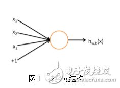
This neuron accepts three inputs x1, x2, x3 and the neuron output is
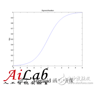
Where W1, W2, W3 and b are the parameters of the neuron, f(z) is called the activation function, and a typical activation function is the Sigmoid function, ie
Its image is
The neural network is a network of multiple neurons. A simple neural network is shown in the figure below.
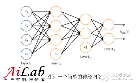
The input of the neural network is represented by a circle, and the circle marked with "+1" is called a bias node, that is, an intercept item. The leftmost layer of the neural network is called the input layer (in this case, there are 3 input cells, the bias cell does not count); the rightmost layer is called the output layer (in this case, the output layer has 2 nodes); The node is called the hidden layer (in this case, there are 2 hidden layers, which contain 3 and 2 neurons, respectively, and the biasing units do not count) because they cannot be observed in the training sample set. Each connection in the neural network corresponds to a connection parameter, and the number of connections corresponds to the number of parameters of the network (in this example, there are 4&Times; 3+4&TImes; 2+3×2=26 parameters). To solve this neural network, a sample set of (x(i), y(i)) is needed, where x(i) is a 3-dimensional vector and y(i) is a 2-dimensional vector.
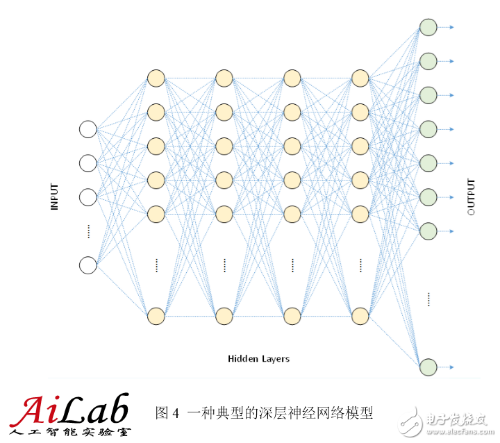
The above figure is a shallow neural network. The following figure is a deep neural network for speech recognition. It has one input layer, four hidden layers and one output layer, and all adjacent two layers of neurons are all connected.
Why is it necessary to construct a deep network structure that contains so many hidden layers? There are some theoretical grounds behind:
3.1 Natural Hierarchical Features
For many training tasks, features have a natural hierarchical structure. Taking voice, images, and text as examples, the hierarchical structure is probably as shown in the following table.
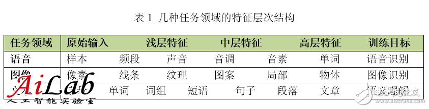
Taking image recognition as an example, the original input of the image is a pixel, adjacent pixels form a line, a plurality of lines compose a texture, a further pattern is formed, and the pattern constitutes a local part of the object until the entire object looks like. It is not difficult to find that we can find the connection between the original input and the shallow features, and then through the middle features, step by step to obtain the connection with the high-level features. It is undoubtedly difficult to get across the high-level features directly from the original input.
3.2 Bionics basis
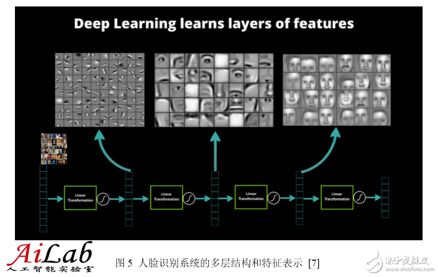
The artificial neural network itself is a simulation of the human nervous system. This simulation has the basis of bionics. In 1981, David Hubel and Torsten Wiesel discovered that the visual cortex is stratified [8]. The human visual system contains different visual neurons. There is a certain correspondence between these neurons and the pupil's stimulus (system input) (the connection parameters between the neurons), that is, after some kind of stimulation ( For a given input, some neurons become active (activated). This confirms that the work of the human nervous system and brain is actually a process of continuously conducting low-level abstractions into high-level abstractions. High-level features are combinations of low-level features, and the higher the feature, the more abstract it is.
3.3 Hierarchical expressibility of features
The hierarchical expressibility of features has also been confirmed. Around 1995, Bruno Olshausen and David Field[9] collected many black-and-white landscape photographs. From these photographs, 400 pieces of 16×16 basic pieces were found. Then some other pieces of the same size were found in the pictures. Fragments are represented as a linear combination of the 400 basic fragments, and the error is as small as possible, using as few fragments as possible. After the representation is completed, fix other debris and select the more appropriate basic debris combination to optimize the approximate result. After repeated iterations, the best elementary fragment combinations that can represent other fragments are obtained. They found that these basic fragment combinations are edge lines of different objects in different directions.
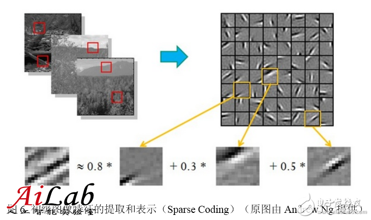
This shows that pixels can be abstracted into more advanced features through effective feature extraction. Similar results apply to speech features.
4 From the shallow model to the deep modelThe previous section talked about the structure of the deep model and its advantages. In fact, deep models have powerful expressive power and can extract high-level features as effectively as humans, and are not new discoveries. So why has the deep model not begun to receive widespread attention and application until recently? Still talking about traditional machine learning methods and shallow learning.
4.1 Shallow model and training methods
Back Propagation (BP algorithm) [10] is a neural network gradient calculation method. The back-propagation algorithm first defines the cost function of the model on the training sample, and then finds the gradient of the cost function for each parameter. The back-propagation algorithm cleverly uses the rule that the gradient of the underlying neuron can be derived from the residuals of the upper neurons. The process of solving is also calculated layer by layer from top to bottom as the algorithm's name, until the gradient of all parameters is obtained. . The back-propagation algorithm can help train statistically based machine learning models, mining statistical rules from a large number of training samples, and then predicting unlabeled data. This kind of statistical learning method has many advantages over traditional rule-based methods [11].
In the 1980s and 1990s, people proposed a series of machine learning models. The most widely used ones include Support Vector Machine (SVM) [12] and Logistic Regression (LR) [13]. Models can be regarded as shallow models containing one hidden layer and no hidden layer, respectively. The back propagation algorithm can be used to calculate the gradient, and then the gradient descent method is used to find the optimal solution in the parameter space. The shallow model often has a convex cost function, the theoretical analysis is relatively simple, the training method is also easy to grasp, and many successful applications have been achieved.
4.2 Training difficulty of deep model
The limitations of the shallow model are limited parameters and computational units. The ability to represent complex functions is limited, and its generalization ability is limited by certain constraints for complex classification problems. The deep model can overcome this weak point of the shallow model precisely. However, applying backward propagation and gradient descent to train the deep model faces several outstanding problems [14]:
1. Local optimum. Different from the cost function of the shallow model, each neuron of the deep model is a nonlinear transform. The cost function is a highly non-convex function. Gradient descent is easy to fall into the local optimum.
2. Gradient dispersion. When using the back-propagation algorithm to propagate gradients, as the depth of the propagation increases, the magnitude of the gradient decreases sharply, causing the weights of the shallow neurons to update very slowly and cannot be effectively learned. In this way, the deep model will become relatively fixed in the first few layers, and only the shallow models of the last few layers can be changed.
3. The ability of the data to obtain a deep model is strong, and the parameters of the model increase accordingly. For training such a multi-parameter model, a small training data set cannot be realized, requiring a large amount of marked data, otherwise it can only lead to severe over fitting.
4.3 Deep Model Training Method
Despite the challenges, Professor Hinton did not give up his efforts. He has been engaged in related research for 30 years and has finally made breakthrough progress. In 2006, he published an article [1] in Science, setting off a wave of deep learning in academia and industry. The two main points of this article are:
1. The multi-hidden layer artificial neural network has excellent feature learning capabilities, and the learned features have a more characterization of the data, which is beneficial for visualization or classification.
2. The difficulty of deep neural network training can be effectively overcome by "Layer-wise Pre-training". An unsupervised layer-wise initialization method is given in this paper.
Excellent feature portrayal capabilities have already been mentioned in the previous article, and are no longer described. The following focuses on the “level-by-layer initialization†method.
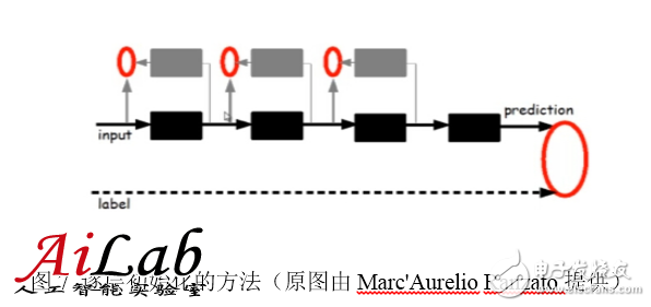
Given the original input, first train the first layer of the model, the black box on the left side of the diagram. The black box can be seen as an encoder that encodes the original input as a primary feature of the first layer and can treat the encoder as a "cognition" of the model. In order to verify that these features are indeed an abstract representation of the input and that there is no loss of too much information, a corresponding decoder, namely the gray box on the left in the figure, needs to be introduced as the "generation" of the model. In order to achieve agreement between cognition and generation, the original input is required to be encoded and then decoded, and it can be roughly restored to the original input. Therefore, the error after the original input and its encoding and decoding is defined as a cost function, while the encoder and the decoder are trained. After training converges, the encoder is the first-level model we want, and the decoder is no longer needed. At this point we get the first level of abstraction of the original data. Fixed the first layer model, the original input is mapped to the first layer of abstraction, as input, such as concocted, you can continue to train out the second layer model, then training the third layer model according to the first two models, and so on, Until the training of the top model.
Once the layer-by-layer initialization is complete, the tagged data can be used to implement the overall supervised training of the model using the back-propagation algorithm. This step can be seen as a fine-tuning of the overall multi-layer model. Since the deep model has many local optimal solutions, the position of the model initialization will largely determine the quality of the final model. The step of "initializing layer by layer" is to make the model in a position that is closer to the global optimum, so as to obtain better results.
4.4 Comparison of Shallow and Deep Models
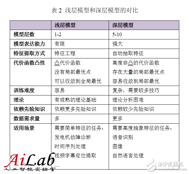
The shallow model has an important feature. It needs to rely on artificial experience to sample the characteristics of the sample. The input of the model is these already selected features. The model is only responsible for classification and prediction. In the shallow model, the most important one is often not the merits of the model, but the merits of the feature selection. Therefore, most people are involved in the development and screening of features. Not only do they need to have a deep understanding of the task problem domain, but they also need to spend a lot of time and effort in trial and error, which also limits the effectiveness of the shallow model.
In fact, layer-by-layer initialization of deep models can also be regarded as the process of feature learning. Through the hidden layer's step-by-step abstract representation of the original input, the original input data structure is learned, more useful features are found, and eventually the classification problem is improved. accuracy. After getting effective features, the overall training of the model can also be achieved.
5 Hierarchical components of the deep modelThe deep model is a neural network that contains multiple hidden layers. What is the specific structure of each layer? This section introduces some common deep model basic hierarchical components.
5.1 Auto-Encoder
A common deep model is constructed by an auto-encoder [6]. The self-encoder can use a set of unlabeled training data {x(1), x(2), ...} (where x(i) is an n-dimensional vector) to perform unsupervised model training. It uses a back-propagation algorithm to get the target value close to the input value. The following figure is an example of an auto encoder:
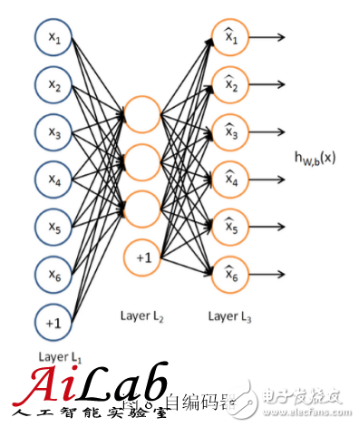
The self-encoder tries to train an identity function so that the output is nearly equal to the input value. The identity function seems to have no learning significance, but considering that the number of hidden layer neurons (in this case, 3) is smaller than the dimension of the input vector (6-dimensional in this case), in fact, the hidden layer becomes a compressed representation of the input data, or a simplified representation of the abstraction. If the input to the network is completely random, compressing high-dimensional vectors into low-dimensional vectors can be difficult to achieve. However, the training data often implies a specific structure, and the self-encoder will learn the correlation of these data and thus obtain an effective compressed representation. After actual training, if the cost function is smaller, the closer the input and output are, the more reliable the encoder is. Of course, since the encoder training is completed, only the previous layer, ie, the encoding portion, is used in actual use, and the decoding portion is useless.
The Sparse Auto-Encoder is a variant of the self-encoder. It adds regularity to the self-encoder. Regularization is to add suppression items to the cost function, hoping that the average activation value of the hidden layer nodes is close to 0. With regularization constraints, the input data can be expressed with a few hidden nodes. Sparse autoencoders are used because sparse expressions are often more effective than dense ones. Human brain systems are also sparsely connected, and each neuron is only connected to a few neurons.
The noise reduction self-encoder is another variant of the self-encoder. By adding noise to the training data, a more robust expression of the input signal can be trained, thereby improving the generalization ability of the model and better coping with the noise that is included in the data during actual prediction.
After getting the encoder, we also want to know more about what we have learned from the encoder. For example, training a sparse auto-encoder on a 10×10 image, and then finding what kind of image for each hidden neuron would allow the hidden neuron to get the maximum incentive, ie what the hidden neuron learned. feature. Finding the features of 100 hidden neurons, we got the following 100 images:
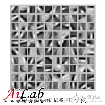
It can be seen that these 100 images have the ability to detect the edges of objects from different directions. Obviously, this ability is very helpful for subsequent image recognition.
5.2 Restricted Boltzmann Machine (RBM)
The Restricted Boltzmann Machine (RBM) is a bipartite graph. The first layer is the input layer (v) and the other is the hidden layer (h). Assume that all nodes are random binary variable nodes. Only 0 or 1 can be used, and it is assumed that the full probability distribution p(v, h) satisfies the Boltzmann distribution.
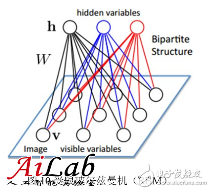
Because there is no connection between nodes in the same layer, in the case of the known input layer, each node in the hidden layer is conditionally independent; conversely, in the case of the known hidden layer, each node in the input layer is also conditionally independent. At the same time, according to the Boltzmann distribution, a hidden layer is generated by p(h|v) when v is input, a hidden layer is obtained, and then an input layer is generated by p(v|h). It is believed that many readers have already guessed that we can adjust the parameters according to similar ideas for training other networks. We hope that the h generated by input v can be generated as close as possible to v, which means that the hidden layer h is the other layer of the input layer v. A representation. This can be used as a basic hierarchical component of a deep model. The deep model entirely formed by RBM is Deep Boltzmann Machine (DBM). If the part near the input layer is replaced by the Bayesian belief network, ie, the directed graph model, and the RBM is still used in the part far from the input layer, it is called Deep Belief Networks (DBN).
5.3 Convolutional Neural Networks (CNN)
The encoders described above are all fully connected networks and can accomplish 10×10 image recognition, such as handwritten digit recognition. However, for larger images, such as 100×100 images, if you want to learn 100 features, you need 1,000,000 parameters and the calculation time will increase greatly. An effective way to solve this size image recognition is to use the locality of the image to construct a partially connected network. One of the most common networks is Convolutional Neural Networks (CNN) [15] [16], which uses the inherent characteristics of the image, that is, the local statistical properties of the image are the same as those of other parts. So the features learned from one part also apply to the other part, and the same features can be used for all locations on this image.
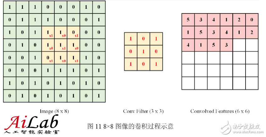
Specifically, suppose you have a 100×100 image from which you want to learn a 10×10 neuron with local image features. If you use a fully connected method, 100×100 dimensions of input to this neuron require 10,000 connections. Weight parameters. With the convolution kernel, only 10 × 10 = 100 parameter weights, the convolution kernel can be seen as a 10 × 10 small window, moving up and down on the image, each 10×10 position in the image (A total of 91×91 locations). Each time a position is moved, the input of the position and the parameter of the corresponding position of the convolution kernel are multiplied and then added up to obtain an output value (an image whose output value is 91×91). The convolution kernel is characterized by a large number of connections, 91 × 91 × 10 × 10 connections, but the parameters are only 10 × 10 = 100, the number of parameters is greatly reduced, training has also become easy, and not easy to produce Fitting. Of course, a neuron can only extract one feature. To extract multiple features, we need multiple convolution kernels.
The following figure shows the schematic process of extracting features using a convolution method for an 8×8-dimensional image. The 3×3 convolution kernel was used. After each 3×3 position in the image, a 6×6-dimensional output image was finally obtained:
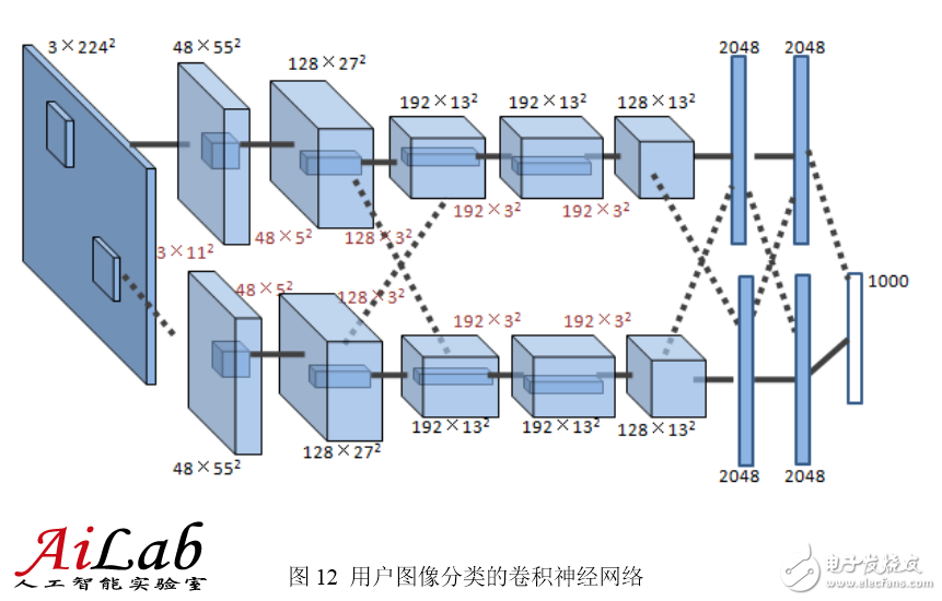
Shown here is a convolutional neural network used by the Hinton research team in the ImageNet competition [2]. There are 5 convolutional layers, each with 96, 256, 384, 384, and 256 convolution kernels, each. The sizes of the convolution kernels are 11×11, 5×5, 3×3, 3×3, and 3×3, respectively. The last two layers of the network are fully connected layers.
6 Deep Learning Training AccelerationDeep model training requires various techniques such as selection of network structure, setting of the number of neurons, initialization of weight parameters, adjustment of learning rate, control of Mini-batch, and so on. Even though these techniques are very proficient, practice must be repeated and tried repeatedly. In addition, there are many parameters in the deep model, the amount of calculation is large, and the scale of the training data is also larger, and it needs to consume a lot of computing resources. If you can speed up training, you can try several new ideas in the same period of time. You can tune several sets of parameters more. The work efficiency will be significantly improved. For large-scale training data and models, you can even more difficult tasks. It becomes possible. This section will talk about the deep model training acceleration method.
6.1 GPU acceleration
Vectorized programming is an effective way to increase the speed of an algorithm. In order to improve the speed of certain numerical operations (such as matrix multiplication, matrix addition, matrix-vector multiplication, etc.), researchers in numerical and parallel computing have worked hard for decades. Vectorization programming emphasizes that a single instruction operates in parallel on multiple similar data to form a single instruction stream multiple data stream (SIMD) programming generic. Deep model algorithms, such as BP, Auto-Encoder, CNN, etc., can be written in vectorized form. However, when executed on a single CPU, the vector operations are expanded into a circular form and are essentially executed serially.
The many-core architecture of GPUs (Graphic Process Units) contains thousands of stream processors, allowing vector operations to be performed in parallel and significantly reducing calculation time. With companies such as NVIDIA, AMD, and others continuing to support the massively parallel architecture of their GPUs, General Purpose-Purpose GPUs (GPGPUs) have become an important means to accelerate parallelizable applications. Thanks to the GPU-many-core architecture, programs run on GPUs at speeds that are several dozen or even thousands of times faster than single-core CPUs. At present, the GPU has developed to a relatively mature stage. The biggest benefit is in the field of scientific computing. Typical successful cases include N-Body Problem, Protein Molecular Modeling, Medical Imaging Analysis, Financial Computing, and Password Computing.
The use of GPUs to train deep neural networks can give full play to the highly efficient parallel computing capabilities of its thousands of computing cores. In scenarios where massive amounts of training data are used, the time spent is drastically reduced, and fewer servers are used. If a proper optimization of the deep neural network is performed, a GPU card can be equivalent to the computing power of dozens or even hundreds of CPU servers, so the GPU has become the industry's preferred solution for deep learning model training.
6.2 Data Parallel
Data parallelism refers to the segmentation of training data. At the same time, multiple model instances are used to train multiple slices of data in parallel.
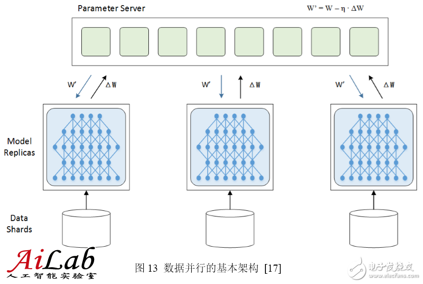
To complete the data parallel, parameters need to be exchanged, which is usually done by a Parameter Server. During the training process, multiple training processes are independent of each other, and the training result, ie, the model change amount ΔW needs to be reported to the parameter server. The parameter server is responsible for updating the latest model W′ = W – η ∙ ΔW, and then The latest model W' is distributed to the training program so that training can be started from a new starting point.
Data parallelism is divided into synchronous mode and asynchronous mode. In the synchronous mode, all training programs simultaneously train one batch of training data, and after completion, they are synchronized and then exchange parameters at the same time. After the parameter exchange is completed, all the training programs have a common new model as a starting point and the next batch is trained. In asynchronous mode, the training program completes a batch of training data and immediately exchanges parameters with the parameter server, regardless of the status of other training programs. The latest results of a training program in asynchronous mode are not immediately reflected in other training programs until they perform the next parameter exchange.
The parameter server is only a logical concept and may not be deployed as a standalone server. Sometimes it is attached to a training program, and sometimes the parameter server is divided into different fragments according to the model and deployed separately.
6.3 Model Parallelism
The model splits the model into several fragments in parallel, which are held by several training units and work together to complete the training. When one neuron's input comes from the output of a neuron on another training unit, communication overhead results.
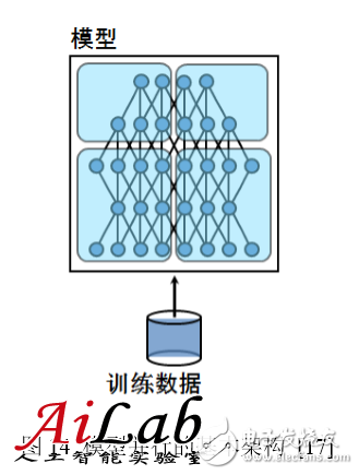
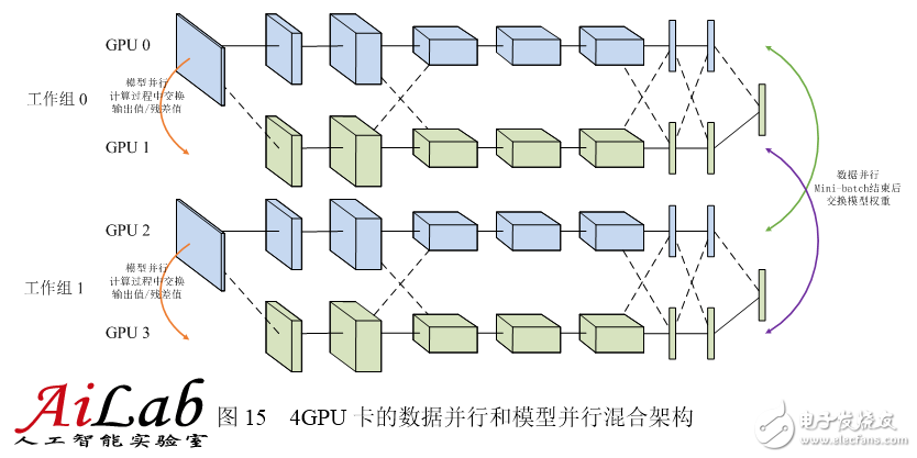
In most cases, the communication overhead and synchronization consumption brought about by the parallelism of the model exceeds the data parallelism, so the speedup ratio is also not parallel to the data. However, model parallelism is a good choice for large models that cannot be accommodated by stand-alone memory. Unfortunately, neither data parallelism nor model parallelism can be infinitely extended. When there are too many data parallel training programs, the learning rate must be reduced to ensure the smoothness of the training process; when the model is divided into too many slices in parallel, the exchange value of the output value of the neuron will increase sharply and the efficiency will drop drastically. Therefore, concurrent model parallelism and data parallelism are also common solutions. As shown in the following figure, the four GPUs are divided into two groups. GPU0, 1 is a group of parallel models, and GPU2, 3 are another group. Each group of models exchanges output values ​​and residuals in parallel during calculation. Data parallelism is formed between the two sets of GPUs, and the model weights are exchanged after the Mini-batch ends. Considering that the blue portion of the model is held by GPU0 and GPU2 and the yellow portion is held by GPU1 and GPU3, only the same color GPU is needed. Exchange weights.
6.4 Computing Cluster
Constructing CPU clusters for deep neural network model training is also a commonly used solution in the industry. Its advantages lie in the use of the powerful computing capacity of large-scale distributed computing clusters, and the use of models for distributed storage and asynchronous communication of parameters to achieve deep training. The purpose of the model.
The basic architecture of the CPU clustering scheme includes Workers for performing training tasks, Parameter Servers for distributed storage distribution models, and Masters for coordinating overall tasks. The CPU clustering solution is suitable for training large models that are difficult to accommodate in GPU memory, as well as sparsely connected neural networks. Andrew Ng and Jeff Dean used 1000 CPU servers at Google to complete deep neural network training of model parallelism and Downpour SGD data parallelism [17].
Combining GPU computing and cluster computing technologies, building a GPU cluster is becoming an effective solution for accelerating large-scale deep neural network training. GPU clusters are built on top of CPU-GPU systems and use more rapid network communication facilities such as 10GbE network cards or Infiniband, as well as logical network topologies such as tree topology. On the basis of the higher computing power of a single node, the collaborative computing capabilities of multiple servers in the cluster are fully exploited to further accelerate large-scale training tasks.
7 Deep Learning Software Tools and PlatformsAt present, there are many mature software tools and platforms for deep learning system implementation.
7.1 Open Source Software
In the open source community, there are the following mature software tools:
Kaldi is a speech recognition tool set based on C++ and CUDA [18][19], which is used by researchers for speech recognition. Kaldi not only implements deep neural network SGD training with a single GPU acceleration, but also implements deep neural network SGD training with CPU multithreading acceleration.
Cuda-convnet is based on C++/CUDA written in deep convolutional neural network using back propagation algorithm [20][21]. Published in 2012 by cuda-convnet, which supports training on a single GPU. Based on its trained deep convolutional neural network model, ImageNet LSVRC-2012 classifies images by 1000 categories and obtains Top 5 classification 15% error rate results [ 2]; The 2014 release supports multi-GPU data parallelism and model parallel training [22].
Caffe provides a fast convolutional neural network implementation on the CPU and GPU, and provides training algorithms. Using NVIDIA K40 or Titan GPUs can complete training for more than 40 million images in a day [23][24].
Theano provides a Python library for deep learning math calculations. It integrates the NumPy matrix computation library, runs on the GPU, and provides good algorithmic extensibility [25][26].
OverFeat is a convolutional neural network system developed by New York University's CILVR Lab. The main application scenario is image recognition and image feature extraction [27].
Torch7 is a scientific computing framework that provides extensive support for machine learning algorithms. The neural network tool package (Package) implements basic modules such as mean squared standard cost function, nonlinear activation function, and gradient descent training neural network. Effortlessly configure the target multilayer neural network to carry out training experiments [28].
7.2 Industrial Platform
In the industry, Google, Facebook, Baidu, Tencent and other companies have implemented their own software framework:
Google's DistBelief system is a data parallelism and model parallelism framework implemented by CPU clusters. It uses tens of thousands of CPU cores to train deep neural network models with up to 1 billion parameters. The main algorithms used by DistBelief are Downpour SGD and L-BFGS. The supported target applications are speech recognition and 21,000 types of image classification [17].
Googleçš„COTS HPC系统是GPU实现的数æ®å¹¶è¡Œå’Œæ¨¡åž‹å¹¶è¡Œæ¡†æž¶ï¼ŒGPUæœåŠ¡å™¨é—´ä½¿ç”¨äº†Infiniband连接,并由MPI控制通信。COTSå¯ä»¥ç”¨3å°GPUæœåŠ¡å™¨åœ¨æ•°å¤©å†…完æˆå¯¹10亿å‚数的深度神ç»ç½‘络è®ç»ƒ[29]。
Facebook实现了多GPUè®ç»ƒæ·±åº¦å·ç§¯ç¥žç»ç½‘络的并行框架,结åˆæ•°æ®å¹¶è¡Œå’Œæ¨¡åž‹å¹¶è¡Œçš„æ–¹å¼æ¥è®ç»ƒCNN模型,使用4å¼ NVIDIA Titan GPUå¯åœ¨æ•°å¤©å†…è®ç»ƒImageNetçš„1000分类网络[30]。
百度æ建了Paddle(Parallel Asynchonous Distributed Deep Learning)多机GPUè®ç»ƒå¹³å°[31]。将数æ®åˆ†å¸ƒåˆ°ä¸åŒæœºå™¨ï¼Œé€šè¿‡Parameter Serveråè°ƒå„机器è®ç»ƒã€‚Paddle支æŒæ•°æ®å¹¶è¡Œå’Œæ¨¡åž‹å¹¶è¡Œã€‚
腾讯深度å¦ä¹ å¹³å°ï¼ˆMarianaï¼‰æ˜¯ä¸ºåŠ é€Ÿæ·±åº¦å¦ä¹ 模型è®ç»ƒè€Œå¼€å‘的并行化平å°ï¼ŒåŒ…括深度神ç»ç½‘络的多GPUæ•°æ®å¹¶è¡Œæ¡†æž¶ï¼Œæ·±åº¦å·ç§¯ç¥žç»ç½‘络的多GPU模型并行和数æ®å¹¶è¡Œæ¡†æž¶ï¼Œä»¥åŠæ·±åº¦ç¥žç»ç½‘络的CPU集群框架。Mariana基于特定应用的è®ç»ƒåœºæ™¯ï¼Œè®¾è®¡å®šåˆ¶åŒ–的并行化è®ç»ƒå¹³å°ï¼Œæ”¯æŒäº†è¯éŸ³è¯†åˆ«ã€å›¾åƒè¯†åˆ«ï¼Œå¹¶ç§¯æžæŽ¢ç´¢åœ¨å¹¿å‘ŠæŽ¨èä¸çš„应用[32]。
8 总结近年æ¥äººå·¥æ™ºèƒ½é¢†åŸŸæŽ€èµ·äº†æ·±åº¦å¦ä¹ 的浪潮,从å¦æœ¯ç•Œåˆ°å·¥ä¸šç•Œéƒ½çƒæƒ…高涨。深度å¦ä¹ å°è¯•è§£å†³äººå·¥æ™ºèƒ½ä¸æŠ½è±¡è®¤çŸ¥çš„难题,从ç†è®ºåˆ†æžå’Œåº”用方é¢éƒ½èŽ·å¾—了很大的æˆåŠŸã€‚å¯ä»¥è¯´æ·±åº¦å¦ä¹ 是目å‰æœ€æŽ¥è¿‘人脑的智能å¦ä¹ 方法。
深度å¦ä¹ å¯é€šè¿‡å¦ä¹ 一ç§æ·±å±‚éžçº¿æ€§ç½‘络结构,实现å¤æ‚函数逼近,并展现了强大的å¦ä¹ æ•°æ®é›†æœ¬è´¨å’Œé«˜åº¦æŠ½è±¡åŒ–特å¾çš„能力。é€å±‚åˆå§‹åŒ–ç‰è®ç»ƒæ–¹æ³•æ˜¾è‘—æå‡äº†æ·±å±‚模型的å¯å¦ä¹ åž‹ã€‚ä¸Žä¼ ç»Ÿçš„æµ…å±‚æ¨¡åž‹ç›¸æ¯”ï¼Œæ·±å±‚æ¨¡åž‹ç»è¿‡äº†è‹¥å¹²å±‚éžçº¿æ€§å˜æ¢ï¼Œå¸¦ç»™æ¨¡åž‹å¼ºå¤§çš„表达能力,从而有æ¡ä»¶ä¸ºæ›´å¤æ‚的任务建模。与人工特å¾å·¥ç¨‹ç›¸æ¯”,自动å¦ä¹ 特å¾ï¼Œæ›´èƒ½æŒ–掘出数æ®ä¸ä¸°å¯Œçš„内在信æ¯ï¼Œå¹¶å…·å¤‡æ›´å¼ºçš„å¯æ‰©å±•æ€§ã€‚深度å¦ä¹ 顺应了大数æ®çš„趋势,有了充足的è®ç»ƒæ ·æœ¬ï¼Œå¤æ‚的深层模型å¯ä»¥å……分å‘挥其潜力,挖掘出海é‡æ•°æ®ä¸è•´å«çš„丰富信æ¯ã€‚强有力的基础设施和定制化的并行计算框架,让以往ä¸å¯æƒ³è±¡çš„è®ç»ƒä»»åŠ¡åŠ 速完æˆï¼Œä¸ºæ·±åº¦å¦ä¹ èµ°å‘å®žç”¨å¥ å®šäº†åšå®žçš„基矗已有Kaldi,Cuda-convnet,Caffeç‰å¤šä¸ªé’ˆå¯¹ä¸åŒæ·±åº¦æ¨¡åž‹çš„å¼€æºå®žçŽ°ï¼ŒGoogleã€Facebookã€ç™¾åº¦ã€è…¾è®¯ç‰å…¬å¸ä¹Ÿå®žçŽ°äº†å„自的并行化框架。
深度å¦ä¹ 引爆的这场é©å‘½ï¼Œå°†äººå·¥æ™ºèƒ½å¸¦ä¸Šäº†ä¸€ä¸ªæ–°çš„å°é˜¶ï¼Œä¸ä»…å¦æœ¯æ„义巨大,而且实用性很强,深度å¦ä¹ å°†æˆä¸ºä¸€å¤§æ‰¹äº§å“å’ŒæœåŠ¡èƒŒåŽå¼ºå¤§çš„技术引擎。
references
[1] Geoffery E. Hinton, Salakhutdinov RR. Reducing the dimensionality of data with neural networks. Science. 2006 Jul 28;313(5786):504-7.
[2] ImageNet Classification with Deep Convolutional Neural Networks, Alex Krizhevsky, Ilya Sutskever, Geoffrey E Hinton, NIPS 2012.
[3] QV Le, MA Ranzato, R. Monga, M. Devin, K. Chen, GS Corrado, J. Dean, AY Ng. Building high-level features using large scale unsupervised learning. ICML, 2012.
[4] Rick Rashid, Speech Recognition Breakthrough for the Spoken, Translated Word?v=Nu-nlQqFCKg
[5] NYU “Deep Learning†Professor LeCun Will Lead Facebook's New Artificial Intelligence Lab.
[6] Stanford deep learning tutorial
[7] A Primer on Deep Learning
[8] The Nobel Prize in Physiology or Medicine 1981.
[9] Bruno A. Olshausen & David J. Field, Emergence of simple-cell receptive field properties by learning a sparse code for natural images. Nature. Vol 381. 13 June, 1996 ~little/cpsc425/olshausen_field_nature_1996.pdf
[10] Back propagation algorithm
[11] 余凯,深度å¦ä¹ -机器å¦ä¹ 的新浪潮,Technical News程åºå¤©ä¸‹äº‹
[12] Support Vector Machine
[13] Logistic Regression
[14] Deep Networks Overview :_Overview
[15] Y. LeCun and Y. Bengio. Convolutional networks for images, speech, and time-series. In MA Arbib, editor, The Handbook of Brain Theory and Neural Networks. MIT Press, 1995
[16] Introduction to Convolutional neural network
[17] Dean, J., Corrado, GS, Monga, R., et al, Ng, AY Large Scale Distributed Deep Networks. In Proceedings of the Neural Information Processing Systems (NIPS'12) (Lake Tahoe, Nevada, United States, December 3–6, 2012). Curran Associates, Inc, 57 Morehouse Lane, Red Hook, NY, 2013, 1223-1232.
[18] Kaldi project
[19] Povey, D., Ghoshal, A. Boulianne, G., et al, Vesely, K. Kaldi. The Kaldi Speech Recognition Toolkit. in Proceedings of IEEE 2011 Workshop on Automatic Speech Recognition and Understanding(ASRU 2011) (Hilton Waikoloa Village, Big Island, Hawaii, US, December 11-15, 2011). IEEE Signal Processing Society. IEEE Catalog No.: CFP11SRW-USB.
[20] cuda-convent https://code.google.com/p/cuda-convnet/
[21] Krizhevsky, A., Sutskever, I., and Hinton, GE ImageNet Classification with Deep Convolutional Neural Networks. In Proceedings of the Neural Information Processing Systems (NIPS'12) (Lake Tahoe, Nevada, United States, December 3–6, 2012). Curran Associates, Inc, 57 Morehouse Lane, Red Hook, NY, 2013, 1097-1106.
[22] Krizhevsky, A. Parallelizing Convolutional Neural Networks. in tutorial of IEEE Conference on Computer Vision and Pattern Recognition (CVPR 2014). (Columbus, Ohio, USA, June 23-28, 2014). 2014.
[23] caffe
[24] Jia, YQ Caffe: An Open Source Convolutional Architecture for Fast Feature Embedding. (2013).
[25] Theano https://github.com/Theano/Theano
[26] J. Bergstra, O. Breuleux, F. Bastien, P. Lamblin, R. Pascanu, G. Desjardins, J. Turian, D. Warde-Farley and Y. Bengio. Theano: A CPU and GPU Math Expression Compiler. Proceedings of the Python for Scientific Computing Conference (SciPy) 2010. June 30 – July 3, Austin, TX.
[27] Overfeat ?id=code:start
[28] Torch7
[29] Coates, A., Huval, B., Wang, T., Wu, DJ, Ng, AY Deep learning with COTS HPC systems. In Proceedings of the 30th International Conference on Machine Learning (ICML'13) (Atlanta, Georgia, USA, June 16–21, 2013). JMLR: W&CP volume 28(3), 2013, 1337-1345.
[30] Yadan, O., Adams, K., Taigman, Y., Ranzato, MA Multi-GPU Training of ConvNets. arXiv:1312.5853v4 [cs.LG] (February 2014)
[31] Kaiyu, Large-scale Deep Learning at Baidu, ACM International Conference on Information and Knowledge Management (CIKM 2013)
[32] aaronzou, Mariana深度å¦ä¹ 在腾讯的平å°åŒ–和应用实践
[33] Geoffrey E. Hinton, Simon Osindero, Yee-Whye Teh, A fast learning algorithm for deep belief nets Neural Compute, 18(7), 1527-54 (2006)
[34] Andrew Ng. Machine Learning and AI via Brain simulations,
https://forum.stanford.edu/events/2011slides/plenary/2011plenaryNg.pdf
[35] Geoffrey Hinton:UCLTutorial on: Deep Belief Nets
[36] Krizhevsky, Alex. “ImageNet Classification with Deep Convolutional Neural Networksâ€. Retrieved 17 November 2013.
[37] “Convolutional Neural Networks (LeNet) – DeepLearning 0.1 documentationâ€. DeepLearning 0.1. LISA Lab. Retrieved 31 August 2013.
[38] Bengio, Learning Deep Architectures for AI, ~bengioy/papers/ftml_book.pdf;
[39] Deep Learning
[40] Deep Learning ~yann/research/deep/
[41] Introduction to Deep Learning.
[42] Google的猫脸识别:人工智能的新çªç ´
[43] Andrew Ng's talk video:
[44] Invited talk “A Tutorial on Deep Learning†by Dr. Kai Yu
â—High-efficiency, energy-saving design, full display of green concept from inside to outside
The system adopts a high-efficiency rectifier, the peak efficiency of the rectifier is greater than 96.2%, and the power consumption of the rectifier sleep is as low as 4W or less.
â—The rectifier module is small in size and high in power density, improving the utilization of cabinet space
â—Fully digital design, more stable performance
The rectifier adopts DSP+MCU dual digital circuit control mode, the system adopts CAN+RS485 dual bus control, the system power supply reliability is higher, and the transmission rate is faster.
High efficiency rectifier
Changzhou Changyuan Electronic Co., Ltd. , https://www.cydiode.com